Plot Linear term

A Linear term maybe penalized exactly like in Ridge regression.

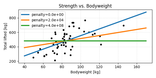
Explained variance (penalty=0.0e+00): 0.352
Explained variance (penalty=2.0e+04): 0.245
Explained variance (penalty=4.0e+08): 0.000

import matplotlib.pyplot as plt
import numpy as np
from generalized_additive_models import GAM, Linear
from generalized_additive_models.datasets import load_powerlifters

rng = np.random.default_rng(42)

# Load data and filter it
df = (
    load_powerlifters()
    .rename(columns=lambda s: s.removeprefix("best3").removesuffix("kg"))
    .sample(50, random_state=42)
)

# Create figure
fig, ax = plt.subplots(1, 1, figsize=(6, 3))
ax.set_title("Strength vs. Bodyweight")
ax.scatter(df["bodyweight"], df["total"], color="black", s=15)

# Loop over penalties
for penalty in [0, 2e4, 4e8]:
    # Fit a GAM with a single Linear term
    gam = GAM(terms=Linear("bodyweight", penalty=penalty))
    gam.fit(df, df["total"])
    score = gam.score(df, df["total"])
    print(f"Explained variance (penalty={penalty:.1e}): {score:.3f}")

    # Plot predictions
    X_smooth = np.linspace(40, 170)[:, None]
    plt.plot(X_smooth, gam.predict(X_smooth), label=f"penalty={penalty:.1e}", lw=3)


ax.grid(True, ls="--", alpha=0.33)
ax.set_xlabel("Bodyweight [kg]")
ax.set_ylabel("Total lifted [kg]")
ax.legend()
fig.tight_layout()
plt.show()