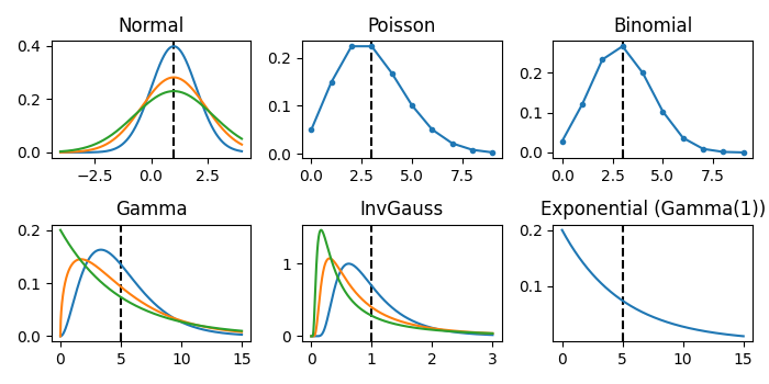
Plot distributions

Plot some of the distributions available.

import matplotlib.pyplot as plt
import numpy as np
from generalized_additive_models.distributions import (
    Binomial,
    Exponential,
    Gamma,
    InvGauss,
    Normal,
    Poisson,
)

fig, axes = plt.subplots(2, 3, figsize=(7, 3.5))
axes = axes.ravel()

# Normal
mu = 1
axes[0].axvline(x=mu, ls="--", color="black")
axes[0].set_title("Normal")
x = np.linspace(-4, 4, num=2**10)
for scale in [1, 2, 3]:
    axes[0].plot(x, Normal(scale=scale).to_scipy(mu).pdf(x))

# Poisson
mu = 3
axes[1].axvline(x=mu, ls="--", color="black")
axes[1].set_title("Poisson")
x = np.arange(10)
axes[1].plot(x, Poisson().to_scipy(mu).pmf(x), "-o", ms=3)

# Binomial
mu = 3
axes[2].axvline(x=mu, ls="--", color="black")
axes[2].set_title("Binomial")
x = np.arange(10)
axes[2].plot(x, Binomial(trials=10).to_scipy(mu).pmf(x), "-o", ms=3)

# Gamma
mu = 5
axes[3].axvline(x=mu, ls="--", color="black")
axes[3].set_title("Gamma")
x = np.linspace(0, 15, num=2**10)
for scale in [0.33, 0.66, 1]:
    axes[3].plot(x, Gamma(scale=scale).to_scipy(mu).pdf(x))

# InvGauss
mu = 1
axes[4].axvline(x=mu, ls="--", color="black")
axes[4].set_title("InvGauss")
x = np.linspace(0, 3, num=2**10)
for scale in [0.33, 1, 2]:
    axes[4].plot(x, InvGauss(scale=scale).to_scipy(mu).pdf(x))

# Exponential - same as Gamma(scale=1)
mu = 5
axes[5].axvline(x=mu, ls="--", color="black")
axes[5].set_title("Exponential (Gamma(1))")
x = np.linspace(0, 15, num=2**10)
axes[5].plot(x, Exponential().to_scipy(mu).pdf(x))

plt.tight_layout()
plt.show()