Under the hood#
Import packages.
[1]:
%load_ext autoreload
%autoreload 2
[2]:
import matplotlib.pyplot as plt
import numpy as np
from generalized_additive_models.datasets import load_salaries

from generalized_additive_models import GAM, Categorical, Spline, Intercept, Linear

rng = np.random.default_rng(42)
/home/docs/checkouts/readthedocs.org/user_builds/generalized-additive-models/envs/latest/lib/python3.11/site-packages/generalized_additive_models/__init__.py:116: UserWarning:
Thank you for using generalized-additive-models, version 0.4.3.
Until version 1.0.0 is released, the package and API should be considered unstable.
You are welcome to use the package. Report bugs and join the discussion on GitHub:
https://github.com/tommyod/generalized-additive-models
  warnings.warn(message)
Load data.
[3]:
df = load_salaries().sort_values("salary")
df[["age", "work_domain", "salary"]].sample(5, random_state=42)
[3]:
| age | work_domain | salary | |
|---|---|---|---|
| 1637 | 58.0 | data science | 950000.0 |
| 1832 | 38.0 | app | 865000.0 |
| 1098 | 23.0 | fullstack | 630000.0 |
| 1172 | 28.0 | backend | 665000.0 |
| 922 | 48.0 | arkitektur | 776000.0 |
Terms are scikit-learn Transformers#
Analogous to Transformers scikit-learn, a term such as Linear implement fit and transform.
Below the age column is transformed by subtracting the mean value.
[4]:
Linear("age").fit_transform(df)
[4]:
array([[33.],
       [23.],
       [33.],
       ...,
       [43.],
       [33.],
       [48.]], shape=(2232, 1))
Categorical variables are one-hot encoded.
[5]:
Categorical("work_domain").fit_transform(df)
[5]:
array([[0., 0., 0., ..., 0., 0., 0.],
       [0., 0., 0., ..., 0., 1., 0.],
       [0., 0., 0., ..., 0., 0., 0.],
       ...,
       [0., 0., 0., ..., 0., 0., 0.],
       [0., 0., 0., ..., 0., 0., 0.],
       [0., 0., 0., ..., 0., 0., 0.]], shape=(2232, 16))
A spline basis is created when we fit and transform using a Spline. Under the hood, the implementation relies on the scikit-learn SplineTransformer. For the visualization to look correct, we must sort the values.
[6]:
X = np.sort(rng.triangular(left=-1, mode=0, right=1, size=2**10))[:, np.newaxis]
plt.figure(figsize=(8, 3))
plt.plot(X.ravel(), Spline(0, num_splines=6).fit_transform(X))
plt.show()
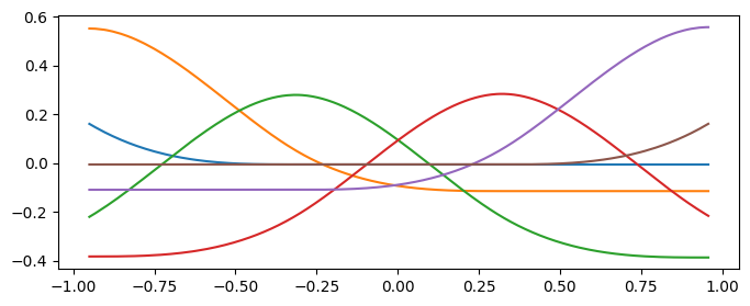
Every spline basis is centered, so the mean value over all data points equals zero.
[7]:
Spline(0, num_splines=6).fit_transform(X).mean(axis=0)
[7]:
array([ 6.91416054e-17, -4.49672851e-17,  2.22966177e-16, -3.44098664e-16,
       -1.02782366e-16, -4.61599075e-17])
[8]:
Spline(0, num_splines=6).fit_transform(X).mean()
[8]:
np.float64(-1.1029216006198245e-17)
Terms may be added#
When we add two Terms, such as Intercept and Linear, a TermList instance is created.
[9]:
terms = Intercept() + Linear("age")
terms
[9]:
Intercept() + Linear(feature='age')In a Jupyter environment, please rerun this cell to show the HTML representation or trust the notebook.
On GitHub, the HTML representation is unable to render, please try loading this page with nbviewer.org.
Parameters
| 0 | Intercept() | |
| 1__by | None | |
| 1__constraint | None | |
| 1__feature | 'age' | |
| 1__penalty | 1 | |
| 1 | Linear(feature='age') |
Fitting and transforming a TermList involves fitting each Term in the TermList.
[10]:
terms.fit_transform(df)
[10]:
array([[ 1., 33.],
       [ 1., 23.],
       [ 1., 33.],
       ...,
       [ 1., 43.],
       [ 1., 33.],
       [ 1., 48.]], shape=(2232, 2))
We can access useful properties, used by the GAM:
[11]:
print("Number of coefficients:", terms.num_coefficients)
print("Penalty matrix:\n", terms.penalty_matrix())
Number of coefficients: 2
Penalty matrix:
 [[0. 0.]
 [0. 1.]]
Penalties (regularization)#
The penalty matrix \(D\) goes into the regulatization term as
[12]:
D = (Intercept() + Linear("age", penalty=2)).penalty_matrix()
D
[12]:
array([[0.        , 0.        ],
       [0.        , 1.41421356]])
The penalty for a Spline acts on the second-order derivative (smoothness) of the spline.
[13]:
Spline(0, num_splines=8).penalty_matrix()
[13]:
array([[ 0.,  0.,  0.,  0.,  0.,  0.,  0.,  0.],
       [ 1., -2.,  1.,  0.,  0.,  0.,  0.,  0.],
       [ 0.,  1., -2.,  1.,  0.,  0.,  0.,  0.],
       [ 0.,  0.,  1., -2.,  1.,  0.,  0.,  0.],
       [ 0.,  0.,  0.,  1., -2.,  1.,  0.,  0.],
       [ 0.,  0.,  0.,  0.,  1., -2.,  1.,  0.],
       [ 0.,  0.,  0.,  0.,  0.,  1., -2.,  1.],
       [ 0.,  0.,  0.,  0.,  0.,  0.,  0.,  0.]])
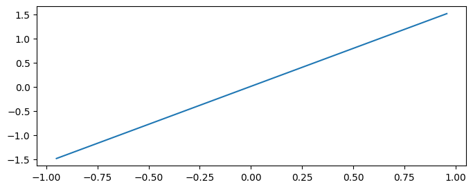
A spline with no smoothness (affine function) results in no penalty.
[14]:
spline = Spline(0, num_splines=6)
beta = np.arange(6)

spline.penalty_matrix() @ beta, np.linalg.norm(spline.penalty_matrix() @ beta)
[14]:
(array([0., 0., 0., 0., 0., 0.]), np.float64(0.0))
[15]:
plt.figure(figsize=(8, 3))
plt.plot(X.ravel(), spline.fit_transform(X) @ beta)
plt.show()
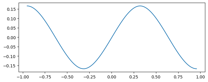
A wiggly, non-smooth spline does incur a penalty.
[16]:
beta = np.array([1, 2, 1, 2, 1, 2])
spline.penalty_matrix() @ beta, np.linalg.norm(spline.penalty_matrix() @ beta)
[16]:
(array([ 0., -2., 2., -2., 2., 0.]), np.float64(4.0))
[17]:
plt.figure(figsize=(8, 3))
plt.plot(X.ravel(), spline.fit_transform(X) @ beta)
plt.show()
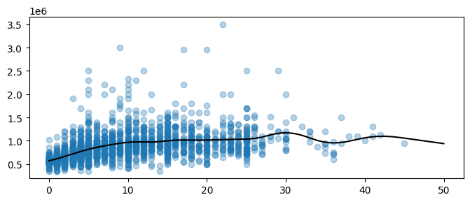
Univariate GAM#
[18]:
model = GAM(Spline("years_relevant_work_experience"), verbose=9)
model.fit(df, df["salary"])
Variables set to zero for identifiability:1/21
Initial guess:      Objective: 1.3762e+14   Coef. rmse: 2.5974e+05
Iteration:  1/100   Objective: 1.3762e+14   Coef. rmse: 2.5974e+05   Step size: 1/2^19
 => SUCCESS: Solver converged (met tolerance criterion).
[18]:
GAM(terms=TermList(data=[Spline(feature='years_relevant_work_experience'), Intercept()]),
    verbose=9)
In a Jupyter environment, please rerun this cell to show the HTML representation or trust the notebook. On GitHub, the HTML representation is unable to render, please try loading this page with nbviewer.org.
Parameters
| terms | TermList([Spl... Intercept()]) | |
| distribution | 'normal' | |
| link | 'identity' | |
| fit_intercept | True | |
| solver | 'pirls' | |
| max_iter | 100 | |
| tol | 0.0001 | |
| verbose | 9 |
Spline(feature='years_relevant_work_experience') + Intercept()
Parameters
| 0__by | None | |
| 0__constraint | None | |
| 0__degree | 3 | |
| 0__edges | None | |
| 0__extrapolation | 'linear' | |
| 0__feature | 'years_relevant_work_experience' | |
| 0__knots | 'uniform' | |
| 0__l2_penalty | 0 | |
| 0__num_splines | 20 | |
| 0__penalty | 1 | |
| 0 | Spline(featur...k_experience') | |
| 1 | Intercept() |
[19]:
years_smooth = np.linspace(0, 50, num=2**10)

plt.figure(figsize=(8, 3))
plt.scatter(df["years_relevant_work_experience"], df["salary"], alpha=0.33)

# Predict with the model
plt.plot(years_smooth, model.predict(years_smooth[:, np.newaxis]), color="black")

plt.show()
[20]:
from sklearn.linear_model import Ridge

spline = Spline("years_relevant_work_experience")
X = spline.fit_transform(df)
y = df["salary"]

ridge = Ridge().fit(X, y)

plt.figure(figsize=(8, 3))
plt.scatter(df["years_relevant_work_experience"], df["salary"], alpha=0.33)
plt.plot(
    years_smooth,
    ridge.predict(spline.transform(years_smooth[:, np.newaxis])),
    color="black",
)
plt.plot
plt.show()

[ ]: