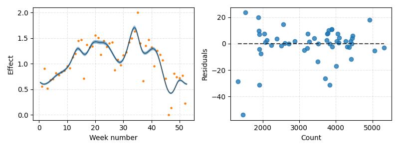
PartialEffectDisplay for Poisson regression

Plot a Poisson regression on a time series dataset.

import matplotlib.pyplot as plt
import pandas as pd
from generalized_additive_models import GAM, Spline
from generalized_additive_models.datasets import load_bicycles
from generalized_additive_models.inspection import (
    PartialEffectDisplay,
    ResidualScatterDisplay,
)

# Load data and filter it
df = load_bicycles()
df = df.loc[lambda df: df.station_name == "Hillevåg", ["date", "count"]]
df = df.assign(date=lambda df: pd.to_datetime(df.date))

# Group by week, choose a single year and get week numbers
df = df.set_index("date").resample("W").sum().reset_index()
df = df[df.date.dt.isocalendar().year == 2019]
df = df.assign(weeknumber=lambda df: df.date.dt.isocalendar().week.values)

# Create periodic spline model
terms = Spline("weeknumber", penalty=1e2, extrapolation="periodic")
gam = GAM(terms=terms, distribution="poisson", link="log")
gam.fit(df, df["count"])

fig, (ax1, ax2) = plt.subplots(1, 2, figsize=(8, 3))

# Partial effect plot
display = PartialEffectDisplay.from_estimator(
    gam,
    gam.terms[0],
    df,
    df["count"],
    ax=ax1,
    residuals=True,  # Plot partial residuals
    standard_deviations=3.0,  # Number of standard deviations
    transformation=True,
)
ax1.grid(True, ls="--", alpha=0.33)
ax1.set_xlabel("Week number")
ax1.set_ylabel("Effect")

# Residual plot - predicted values vs residuals
ResidualScatterDisplay.from_estimator(
    gam, df, df["count"], residuals="deviance", ax=ax2
)
ax2.grid(True, ls="--", alpha=0.33)
ax2.set_xlabel("Count")

plt.tight_layout()
plt.show()