ResidualScatterDisplay

Plot a Gaussian regression on a dataset with powerlifters.

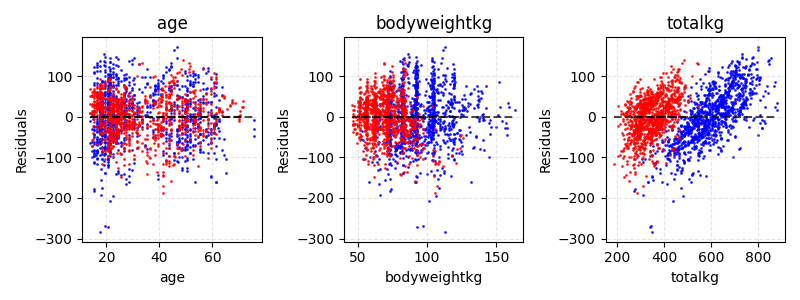
Explained variance: 0.8568129733333859

import matplotlib.pyplot as plt
from generalized_additive_models import GAM, Categorical, Spline
from generalized_additive_models.datasets import load_powerlifters
from generalized_additive_models.inspection import ResidualScatterDisplay

# Load data and filter it
df = load_powerlifters()

# Predict total weight lifted, given age, bodyweight and sex
target = df["totalkg"]
age = Spline("age")
bodyweight = Spline("bodyweightkg")
sex = Categorical("sex")

terms = age + bodyweight + sex
gam = GAM(terms=terms, distribution="normal", link="identity")
gam.fit(df, target)

print("Explained variance:", gam.score(df, target))

fig, axes = plt.subplots(1, 3, figsize=(8, 3))

for feature_name, ax in zip(["age", "bodyweightkg", "totalkg"], axes.ravel()):
    ax.set_title(feature_name)

    # Split the plot based on the categorical variable
    for sex, color in zip(["M", "F"], ["blue", "red"]):
        df_subset = df[df.sex == sex]
        residuals = gam.residuals(
            df_subset, df_subset["totalkg"], residuals="deviance", standardized=False
        )

        viz = ResidualScatterDisplay(x=df_subset[feature_name], residuals=residuals)
        viz.plot(ax=ax, scatter_kwargs={"s": 1, "color": color, "alpha": 0.8})

    ax.set_xlabel(feature_name)
    ax.grid(True, ls="--", alpha=0.33)

plt.tight_layout()
plt.show()