Getting started#
Import packages.
[1]:
import matplotlib.pyplot as plt
import numpy as np
from sklearn.datasets import load_diabetes

from generalized_additive_models import GAM, Categorical, Spline
/home/docs/checkouts/readthedocs.org/user_builds/generalized-additive-models/envs/stable/lib/python3.11/site-packages/generalized_additive_models/__init__.py:116: UserWarning:
Thank you for using generalized-additive-models, version 0.4.3.
Until version 1.0.0 is released, the package and API should be considered unstable.
You are welcome to use the package. Report bugs and join the discussion on GitHub:
https://github.com/tommyod/generalized-additive-models
  warnings.warn(message)
Load data.
[2]:
data = load_diabetes(as_frame=True)
df = data.data
y = data.target

# Code the "sex" variable as strings
df = df.assign(sex=lambda df: np.where(df.sex < 0, "Male", "Female"))

df.sample(5)
[2]:
| age | sex | bmi | bp | s1 | s2 | s3 | s4 | s5 | s6 | |
|---|---|---|---|---|---|---|---|---|---|---|
| 163 | 0.016281 | Female | 0.072474 | 0.076958 | -0.008449 | 0.005575 | -0.006584 | -0.002592 | -0.023647 | 0.061054 |
| 95 | -0.070900 | Male | -0.057941 | -0.081413 | -0.045599 | -0.028871 | -0.043401 | -0.002592 | 0.001148 | -0.005220 |
| 298 | 0.023546 | Female | -0.037463 | -0.046985 | -0.091006 | -0.075530 | -0.032356 | -0.039493 | -0.030748 | -0.013504 |
| 192 | 0.056239 | Female | -0.030996 | 0.008101 | 0.019070 | 0.021233 | 0.033914 | -0.039493 | -0.029526 | -0.059067 |
| 275 | -0.005515 | Female | -0.011595 | 0.011544 | -0.022208 | -0.015406 | -0.021311 | -0.002592 | 0.011011 | 0.069338 |
Creating a model#
Construct and fit a model.
[3]:
# Features can be string and refer to column names if X is a pandas DataFrame
# If X was a 2D numpy array, features must instead be integers referring to the columns

terms = Spline("age") + Categorical("sex", penalty=1) + Spline("bmi") + Spline("bp")
model = GAM(terms, link="identity", verbose=2, fit_intercept=False)

# Fit the model
model.fit(df, y)
Variables set to zero for identifiability:3/62
Initial guess:      Objective: 1.5233e+06   Coef. rmse: 1.1671e+02
Iteration:  1/100   Objective: 1.5233e+06   Coef. rmse: 1.1671e+02   Step size: 1/2^19
 => SUCCESS: Solver converged (met tolerance criterion).
[3]:
GAM(fit_intercept=False,
    terms=TermList(data=[Spline(feature='age'), Categorical(feature='sex'), Spline(feature='bmi'), Spline(feature='bp')]),
    verbose=2)
In a Jupyter environment, please rerun this cell to show the HTML representation or trust the notebook. On GitHub, the HTML representation is unable to render, please try loading this page with nbviewer.org.
Parameters
| terms | TermList([Spl...eature='bp')]) | |
| distribution | 'normal' | |
| link | 'identity' | |
| fit_intercept | False | |
| solver | 'pirls' | |
| max_iter | 100 | |
| tol | 0.0001 | |
| verbose | 2 |
Spline(feature='age') + Categorical(feature='sex') + Spline(feature='bmi') + Spline(feature='bp')
Parameters
| 0__by | None | |
| 0__constraint | None | |
| 0__degree | 3 | |
| 0__edges | None | |
| 0__extrapolation | 'linear' | |
| 0__feature | 'age' | |
| 0__knots | 'uniform' | |
| 0__l2_penalty | 0 | |
| 0__num_splines | 20 | |
| 0__penalty | 1 | |
| 0 | Spline(feature='age') | |
| 1__by | None | |
| 1__feature | 'sex' | |
| 1__handle_unknown | 'error' | |
| 1__max_categories | None | |
| 1__min_frequency | None | |
| 1__penalty | 1 | |
| 1 | Categorical(feature='sex') | |
| 2__by | None | |
| 2__constraint | None | |
| 2__degree | 3 | |
| 2__edges | None | |
| 2__extrapolation | 'linear' | |
| 2__feature | 'bmi' | |
| 2__knots | 'uniform' | |
| 2__l2_penalty | 0 | |
| 2__num_splines | 20 | |
| 2__penalty | 1 | |
| 2 | Spline(feature='bmi') | |
| 3__by | None | |
| 3__constraint | None | |
| 3__degree | 3 | |
| 3__edges | None | |
| 3__extrapolation | 'linear' | |
| 3__feature | 'bp' | |
| 3__knots | 'uniform' | |
| 3__l2_penalty | 0 | |
| 3__num_splines | 20 | |
| 3__penalty | 1 | |
| 3 | Spline(feature='bp') |
[4]:
model.summary()
| Property           | Value      |
|--------------------|------------|
| Model              | GAM        |
| Link               | Identity() |
| Distribution       | Normal     |
| Scale              | 3574.069   |
| GCV                | 3854.516   |
| Explained deviance | 0.441      |

| Term             |   Coefs |   Edof |
|------------------|---------|--------|
| Spline(age)      |      20 | 10.381 |
| Categorical(sex) |       2 |  1.99  |
| Spline(bmi)      |      20 |  9.754 |
| Spline(bp)       |      20 | 10.035 |

| Term                    |    Coef |   Coef std |
|-------------------------|---------|------------|
| Categorical(sex=Female) | 146.735 |     4.3758 |
| Categorical(sex=Male)   | 155.602 |     4.083  |
Make a prediction and score the model.
[5]:
predictions = model.predict(df)
model.score(df, y)  # Pseudo R2 score
[5]:
np.float64(0.4411312994129862)
Since this model has a normal distribution and an identity link, the score equal the R2 score.
[6]:
from sklearn.metrics import r2_score

r2_score(y_true=y, y_pred=predictions)
[6]:
0.44113129941298623
Scikit-learn compatibility#
The models interact nicely with scikit-learn.
[7]:
from sklearn.model_selection import cross_val_score

# Models can be used with sklearn's `cross_val_score`
model = GAM(Spline("bp"))
cross_val_score(model, df, y, scoring="r2")
[7]:
array([0.07107161, 0.16072369, 0.15168224, 0.18885055, 0.25517882])
[8]:
from sklearn.model_selection import GridSearchCV

model = GAM(Spline("bp"))

# A parameter grid can be used to search for e.g. the best spline penalty
param_grid = {"terms__penalty": [1, 10, 100, 1000]}
search = GridSearchCV(model, param_grid, scoring="r2").fit(df, y)
search.best_params_
[8]:
{'terms__penalty': 100}
[9]:
# To search over more than one term, use a `param_grid` like this
model = GAM(Spline("bp") + Spline("age"))

# The integers are used to index the terms, so 0 refers to the first term, etc
param_grid = {
    "terms__0__penalty": [1, 10, 100, 1000],
    "terms__1__penalty": [1, 10, 100, 1000],
}
search = GridSearchCV(model, param_grid, scoring="r2").fit(df, y)
search.best_params_
[9]:
{'terms__0__penalty': 100, 'terms__1__penalty': 1000}
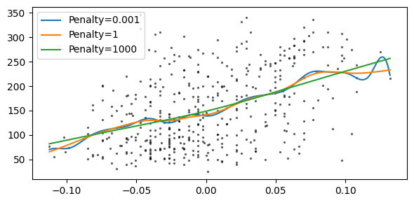
Penalties#
[10]:
plt.figure(figsize=(6, 3))
plt.scatter(df["bp"], y, s=2, alpha=0.5, color="k")

X_smooth = np.linspace(df["bp"].min(), df["bp"].max(), num=2**10).reshape(-1, 1)

for penalty in [0.001, 1, 1000]:
    model = GAM(Spline("bp", penalty=penalty)).fit(df, y)

    plt.plot(X_smooth, model.predict(X_smooth), label=f"Penalty={penalty}")

plt.legend()
plt.tight_layout()
plt.show()